Saturday, May 26, 2018

Christopher Columbus and the Spherical Earth

Columbus has long been a pet peeve of mine. I regret the unfounded adulation he is given in schools, which seems to persist into public thoughts on him. He would be better remembered as the founder of the African slave trade between Europe and the Americas—although I can say that in the city of Seattle, Columbus Day has been officially changed to Indigenous Peoples Day.

Reading his log, we find that Columbus was indeed a true master at ocean dead reckoning, which in the day was the key to good navigation, as it remains today. But that is the end of what good we can say about him. He was a charlatan, motivated by religious dogma and personal greed... but I digress.

He believed the flat earth theory promoted by the church at a time that every educated person in Europe knew the earth was a sphere, and many knew the circumference of it, which was measured remarkably accurately in 250 BC (see end notes here). In writing about Columbus in numerous places, I have made that statement, and just moved on. Today, cleaning up the office—a regular routine here carried out every two or three decades—I ran across a folder I had made in the early 90s, showing roman coins depicting a globe, which were at one point gathered to support that argument. So now with the convenience of the blogosphere, I present these below and throw away the old prints as a step in cleaning house. They are apparently from a coin collectors catalog.

In other words, the concept of the earth as a spherical globe was so well known in Roman times that it appeared on common coins.


To supplement this thought, here is a figure from our Celestial Navigation text explaining the first accurate measurement of the size of the earth... which I just realized now, has another of my digs at Columbus! 

The measurement relies on basic principles of celestial navigation, known in 250 BC, but much expanded upon by 1490—when Columbus was traipsing around with some obscure map based on a religious cult that he did not know how to interpret. Needless to say, many people of his time and for another 300 years, wise and unwise, were overly influenced by the church, but they did not go as far as Columbus did to risk this voyage so he could get rich enough to fund his own crusade. They did not tell me about that in school.


Figure 10.3-3.  How Eratosthenes measured the circumference of the earth in about 250 BC. On the solstice he knew the sun was overhead in Syene (Aswan, 24º 4’N, 53º 7’E), as the sun was known to shine directly down deep wells. It was also known that in Alexandria, 428 nmi to the north, on the same day at noon there were indeed shadows cast by the midday sun. He measured the sun’s zenith distance of 7.2º there at that time, probably from the length of a shadow as shown. The distance between these two cities was well known at the time. Since the measured angle turned out to be 1/50th of a full circle, the full circle must be 50 × the distance between the cities.

We are not sure exactly how well he knew it at the time, but we now know there is 428 nmi of latitude between these two cities. This gives a result that is almost spot on the right circumference. Celestial navigators know the circumference of the earth automatically, because of the definition of a nautical mile, namely: 360º × 60 nmi/1º, or 21,600 nmi.

The main uncertainty in figuring his exact accuracy stems from not knowing the exact definition of his unit of length. Using all variations of this and accounting for the offset to the west of Alexandria, his error was somewhere between 0.1% and 16%. In any case, very good. The factor of exactly 1/50th is just a numerical accident from the geometry of the measurement.

What is rather more curious than the greatness of this achievement—Eratosthenes had so many, in various sciences—is that Columbus was totally oblivious to this information 1240 years later. Other navigators before Columbus and after him were well aware of the dimensions of the earth. It was not long after Columbus’s voyages that this knowledge all resurfaced and world charts proliferated.

Syene had been a famous city in Egypt, long before the Aswan dam. Since ancient times it was the southern frontier, located at the first cataracts that blocked farther navigation of the Nile to the south. It was a 3 to 4 week sail from Syene to Alexandria. The stones of the pyramids were quarried near there and shipped north.


Tuesday, May 15, 2018

Paper Charts vs. Electronic Charts — Some Thoughts

This is an outline of a talk given at Captain's Nautical Supply on May 15, 2018 in support of the Coho HoHo program. 

Those reading online will need to do some reading between the lines... or better still, get a copy of our book on the subject! 

_________________

• These days there is no reason not to have every chart we might ever want stored on our computers, tablets, or even phones.

• Tablets are handy, but we can still do very much more with a computer.

• Generally PCs are still more functional than Macs for navigation and weather... the only exception is LuckGrib.com for Mac, which also has an iOS version for PC users with an iPad. This is the state of the art GRIB source and viewer without parallel, on any platform. Mac or iOS costs $20. (I have no financial ties to this product, but am a strong proponent... if you care about weather, it will change your life!)

• Main reference: Introduction to Electronic Chart Navigation. This is a unique resource with information not found in other sources. Crucial to successful use of ENC.


Main value of electronic chart systems (ECS) over paper charts 

• Boat position tracks on the chart, as well as AIS targets

Prior to live GPS tracks on our chart screen (ie ECS), navigators were always finding where the boat was some time ago, since it takes time to plot out the piloting fix during which the boat is moving. A main revolution of ECS is we now know where the boat is on the chart at the moment.

• CPA can be displayed on most ECS (electronic charting systems)

• Depth, obstructions, and other alarms can be set on vector charts.

• Layout routes and compute route table (leg distances, headings, times, names)

• Shows tides and currents. We still have the obligation to check our results periodically.

• Quick range and bearing lines for piloting

• Easy to keep charts up-to-date

• In US waters and other places as well, charts are free whereas paper charts always expensive

• Usually easier to see in various conditions (bright light on the deck is an exception)

• Vector charts have more detail than paper charts


Main value of paper charts over echarts

• They work when they are wet.

• They don't require power.

• The view is always the same and cannot be screwed up by wrong device settings, or a mis-click at a crucial time.  (Generally tricky situations are best navigated with echarts, with the best paper chart laid out on the chart table.)

• Anyone on the boat can walk up to the chart table and understand what they are seeing; they do not need to turn on a computer or be trained in the use of the ECS.

• As such, a minimum number of paper charts are still required for any voyage. When all traditional paper charts are gone (end of 2024), we will make the paper charts we need from the new NOAA Custom Chart (NCC) program.


Overview of our resource starpath.com/getcharts

• For echarts and paper charts

• Check out the interactive viewer for chart selection

• Check out seamless ENC viewer to see how ENC charts work... i.e., click an object.

• Check out pdf charts... they can be stored in your phone or tablet. They will be discontinued one for one with the paper charts. 


Using ENC (electronic navigational charts) 

compared to 

RNC (raster navigational charts)

• See Fig 1.2-1  [ Figure references are to our electronic charts book above ]


• See also Fig 2.6-2


• ENC require an all new approach to chart reading.

• User controls what is shown on the chart (Base, Standard, Custom).

• User controls the scale of the chart, which is done with RNC as well, but this is more consequential and effective  with ENC.

• All objects have an attribute SCAMIN, which is the smallest scale the object will be displayed upon. This is a subtly to be reckoned with. A light with SCAMIN 21999, for example, will show when the display is zoomed to 1:20,000, but will not show if you zoom out to 1:23,000. This feature of ENC can be overridden by user controls in most programs.

• qtVlm and OpenCPN has an excellent presentations of the S-52 format (the official  ENC presentation standard)

• Descriptions of many symbols are not printed on the chart, but all are included in object and attribute descriptions accessed by a "cursor pick."  Users can usually control the amount of labels to be shown.

• Everything on the chart is an object, which has attributes, one of which is often a category, which in turn has a list of options.  See sample in Table 1.7-4. Check links below to see more.


• All objects and attributes are assigned a 6-letter abbreviation i.e., UWTROC. The IHO calls these acronyms, but they are not. 

• These descriptions are in our Appendix, but also online at  www.caris.com/s-57   Another source online with a different layout is www.s-57.com  This one is based in Russia and we are told may not always be up to date, but sometimes its layout makes it easier to find something... also these values do not change very often. These can be called "online ENC object catalogs."

Where have all the towers gone?  There are no towers on ENC. They are now an object LNDMRK, with attribute CATLMK = tower, with maybe a function (FUNCTN) specified, such as radio tower.  See other attributes of LNDMRK at one one of the online object catalogs for details.

• Chart names of ENC are different and convey more info that those of RNC. The forthcoming re-schemed ENC include even more information in the chart names. This ENC conversion process is well underway at the moment.

• Regions covered by specific ENC are irregular and do not correspond directly with RNC.  See Fig. 1.5-1 and Table 1.5-2.  These irregular borders are the main thing being changed in the rescheming program.


• Safety depth zones can be defined to match the vessel. See Figures 2.4-1a and 2.4-1b.


Special Value of ENC

• More info on the chart. Objects have more specifications, and this will just improve with time, plus they effectively include all Light List data.

• Alarms on obstructions and depths are automatic,  whereas if needed on RNC we have to define boundaries.

• Cleaner view of some areas, with options to "over zoom" in productive ways.

• US ENC one of the few that do the height datum contour correctly. Can use it to read MHW. See Figure 2.8-2.  The renowned UKHO ENC do not do this properly!  Canadian ENC are even worse on this detail, though both are otherwise fine sources of ENC.


• File size for storage and update delivery is much smaller than RNC. (Once activated in your nav program this is less of a factor, because the ENC size gets doubled when creating the necessary SENC files, but even doubled they are notably smaller.)

• Looking ahead, the new S-412 weather overlays planned by the NWS will be so powerful that we will be forced to use ENC just to access that program.  See discussion in our new book Modern Marine Weather, 3rd ed.


Wednesday, May 9, 2018

Ocean Rowboat Polar Diagram

Ocean rowing is a growing sport. This year the Great Pacific Rowing Race will be sharing the race course to Hawaii with both the Pacific Cup and Vic-Maui sailboat fleets. The dynamics of rowing are of course very different from sailing, but it occurs to me that we might do some form of optimum routing for the rowboats as we do routinely for sailboats.

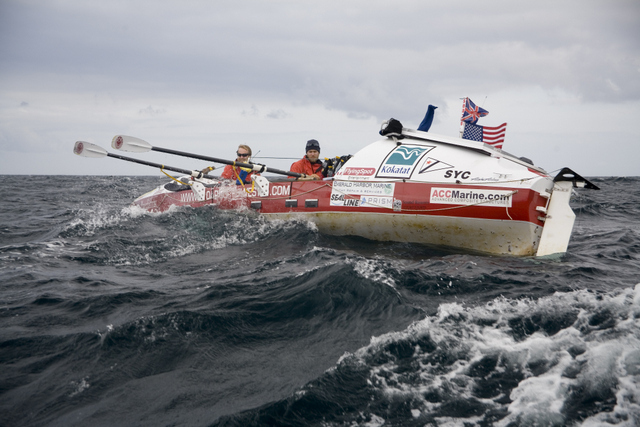
Figure 1. Start of the 2014 Great Pacific Rowing Race. Photo by Ellen Hoke Photography. This shows the type of boats we are discussing, sometimes called "classic fours." Crew of four, rowing two at a time, about 30 ft long, about 3,000 lbs fully loaded for a crossing.

As it turns out, wind is as important to ocean rowboats as it is to sailboats, and ocean currents are proportionally more important. We have all the tools in place from the sailboat technology to compute an optimum route, providing we can come up with some reasonable set of rowboat polar diagrams.

I have been working with my friend Jordan Hanson and his OAR Northwest rowing projects for many years, starting with assisting them on their record-setting 2006 transatlantic victory, NYC to Falmouth, England. They also rowed around Vancouver Is, which is frankly as challenging on the outside leg as being in the North Atlantic—actually more so, because there is a rocky coast on one side of them. In 2013, he and his team rowed from Dakar, Senegal to just north of Puerto Rico, where an unusual back to back sequence of big waves flipped the boat during a watch change when a hatch was open. All were rescued, and in another feat of seamanship and perseverance Jordan followed up with an air search and subsequent tugboat rescue of the boat itself.

He and his team have also rowed around the Olympic Peninsula, a complete circumnavigation by row
boat. Yes, there is indeed water on all sides of this large section of our state... something that we at Starpath confirmed years ago.

What we have below is a compilation of his thoughts on this matter for a classic fours as we discussed it. We propose this as a starting point to build from. These days with all the sophisticated data logging possible, we should be able to home in on this fairly well. The upcoming row race that starts on Jun 2 will be online, tracked by YellowBrick. We also have Jordan's Logbook from the 2006 trip and the training for it. That includes wind speed and direction, discussion of waves, along with COG and SOG, although actual numbers from that data were not used here—that is on the list to do.

We make these assumptions:

(1) We consider two rowing speed limits. A boat that can row steadily, over long periods in flat water and no wind, with an average speed of 1.5 kts and a boat that can average 2.5 kts in these same conditions. Most boats will be somewhere between these two limits.

(2) We are predicting the average speed made good (SMG) over a long period, several hours or more. These boats can surf down big waves at up to 10 kts or so, but these are just very short bursts.

(3) We assume here that the wind has been blowing long enough at the given speeds that the seas have built to their typical potential for each wind speed. This won't necessarily be fully developed seas, but just typical of what you might see. (This is a different approach from sailboat routing where we consider effect of wind and waves separately.)

(4) We assume the wind and waves are in the same direction. It is likely fair to assume that the SMG will be lower when these two differ by 45º or more.

(5) We assume for now that we can base the full range of wind angles on vector components of the estimates for head winds and tail winds alone.

And we come up with Figure 2.

Figure 2. Estimates of rowing speeds vs. wind speeds.

Sailors will have to pause a moment when looking at this!  It looks a lot different than what we are used to.  Boats that row 1.5 to 2.5 kts in flat water will be assisted by tail winds quite notably. The issue here is momentum. The boats weigh some 3,000 lbs, so it is work to get them going, but once moving, they can be kept moving with less effort, which is notably assisted with wind behind them. With a sustained wind behind them of just 15 kts, the average speed, with about the same effort, goes up some 40%. This gain increases with wind speed up till there is a physical limit on steering the boat. At some point around 20-25 kts, it can be more efficient to give up, set out a sea anchor, and just drift with this tail wind in the right direction.

The amount they slow down on the sea anchor depends on the diameter of the anchor. Jordan's experience is mostly with a 9-ft model, which he says really stops the boat, leaving it drifting at some 1 kt or so. A smaller sea anchor would let them drift faster, which we have estimated in the diagram above.  This is just one aspect of this preliminary analysis that we await more input on.  We assume that by 25 kts most boats would opt for the extra rest rather than the fight to steer the boat.

Rowing into the wind, they get stopped at lower wind speeds.  Here we guess that some boats might fight it up to 17-20 kts, but at some point, again, the effort is not worth the value of rest.

With wind on the nose, when you stop rowing and set the sea anchor, you start drifting backwards, so your SMG is negative. In this case the bigger the sea anchor the less you lose. (Do boats carry sea anchors of different sizes?)

With these starting point estimates, we then look at wind at other angles, using the logic of Figure 3.


Figure 3. Estimating effect of TWS at various TWA based on head-wind and tail-wind values. For example, with a TWS of 10 kts at a TWA = 45, we would read the effect on the boat from Figure 2 using a TWS of 7 kts. 

We break the wind up into either a head-wind or tail-wind component and a leeway component, which in this first analysis, we assume does not affect forward speed.  With this assumption, a beam wind does not slow down forward progress, but just makes it harder to row. On closer look, this might end up being a negative number near the beam, if the rowers can only keep one oar in the water at a time. Again, we wait for feedback on this.

Figure 4. Wind on the beam. Jordan's 2006 crossing.

This simple model implies that if with 15 kts of wind on the stern you make good 3.5 kts, then with 15 kts on the quarter (relative bearing 135º) you would enter Figure 2 with 0.7x15 = 10.5 kts and find a SMG of about 2.8 kts.

Likewise, if 15 kts on the nose has slowed you to 1.0 kts, then 15 kts of wind on the bow (relative bearing 45º), enter the table with 10.5 kts to get a SMG of about 1.5 kts.

If this logic makes sense, then we can create the polars for all TWA and TWS.  Each boat would then have a set of curves for SMG vs TWS and TWA depending on their starting point at TWS = 0. But before getting out the spread sheets, we wait for comments here to confirm or propose changes to this crude  model.

Ocean rowboat routes are largely downwind (Figure 5), which can be seen by looking at the Yellowbrick tracks of past races along with the prevailing weather maps at the time. But there will certainly be times in a race where one might want to work toward a desired route, and indeed if this analysis works out, we should be able to compute when that is best done.  If the polars are right, the routing programs will tell us that.

Figure 5. July COGOW scatterometer winds as presented by Pitufa, overlaid with the 2014 routes from the Great Pacific Row Race site. The 2016 routes are about the same. The goal at hand is to figure how much a rower should strive for the best route when it does not follow the winds around the Pacific High route.

Needless to say, we face the same challenge of sailors in that the forecasts are good for a few days but then get progressively less reliable.  We can, for example, get 16 days of GFS wind forecasts, which would make an interesting test for the rowboat routing computation.  The wind forecasts are not dependable after 4 or 5 days, but they will be something to start with, and the amount the forecasts drift off of correct is more important to sailboats than to rowboats. So this too adds some confidence to this approach.

The working procedure with these tactics is you run the optimization computation every 6 hr when the new forecasts come out. We cover the ways to evaluate these computations while doing them in our newly released Modern Marine Weather, 3rd ed. The routes compute in seconds, so we can try lots of variations.  There are several high quality routing programs for iPad or Android tablets, and the wind data can be downloaded by satphone while underway. Predictwind offers a service of computing the routes for you based on your polar diagrams stored with your account info. You send the request (departure, destination, and start time) by email and they return the route by email.

Standing by...

Tuesday, May 8, 2018

Ways to Get Accurate GMT (UTC)

Celestial navigation is one of the few human endeavors that requires us to know the time accurate to the second. In earlier days of celestial navigation—which for the purposes at hand we can say means more than thirty years ago—this was more or less easily accomplished by HF radio broadcasts, but in these modern days of the Internet, cell phone networks, and ubiquitous GPS, it is now very much easier.

That does not distract, by the way, from the high value of having a good old fashioned watch on board whose rate we monitor frequently. A modern justification for learning cel nav after all is to be independent of electronics for ocean navigation, and we need to know the time to do cel nav well... or at least efficiently. Put another way, you can sail around the world fairly efficiently from port to port with nothing at all but a watch (and some books and knowledge), but take away any time piece and it will be difficult to DR for 100 miles. Our textbook Celestial Navigation has extended sections on time keeping in navigation.

Thus if you have a watch for navigation, you will need some way to check it frequently so you can establish its rate, ie how many seconds it gains or loses every week or so.  A typical quartz watch is 15 to 20s/month and they are not as well temperature compensated. But we need some way to test that this is really true, so we show below here four independent ways to get accurate GMT.

In principle any one method would do, and one could just list what the methods are, but unless you see them side by side, then that would have to be taken on faith—a type of justification we try to avoid in navigation whenever possible.

Here are the methods

(1) Tune in an HF (SW) radio to one of the international frequencies that broadcast time tics. These are listed in Radio Aids to Navigation, the applicable chapter we have online at this link.  The best known and most often used of these is WWV and WWVH at 5, 10, 15, 20 MHz.

(2) Call this phone number to hear the WWV broadcast on your phone: (303) 499-7111. This is a great trick, and it would seem that navigators might want to have this number in their contacts list.

(3) Logon to www.time.gov and select UTC and see the time presented for you. You will see their note that the displayed time is "Corrected for network delay."

(4) Use any GPS that is connected to satellites and giving an active location to find the display that will also show the UTC.  Note that the GPS will turn on without satellite connections and indeed might even tell you the time, but this is not dependable without the actual connection.

(5) Read your cell phone time.  When you are connected to a network the phone should give you the correct time. Note that strangely enough, the iPhones do not have a native display of time accurate to the second, but there are numerous free apps that read it and then show the time to the second. I should also note that i have seen rare instances when the cell phone time was off a few seconds over a period of several minutes, but I do not know what might be the source of this.  The primary source of time in the phones is the network providers, which are in principle getting the time from GPS.

(6) Most modern computers are designed to show the network time whenever you are logged on to the Internet.  If you are some period of time off line, then the computer could drift, but if you have a wireless connection, your computer should be showing the right time.

Here is a video showing the whole band playing at once... in keeping with our totally non-professional standards of production.


Here is an example for finding watch rate by recording watch time and correct time. First set the watch and then every few days record its error, to get a table like this one:

from this we can make a plot as shown below.


Figure 11.5-2. Chronometer log plots. Top is an inexpensive quartz watch, which is slow, showing a rate -3.5s/10d. Bottom is a $600 watch with a guaranteed rate of <10s/year (dashed lines), but actual rate was +1.1s/10d, which shows we need to check these things. Bottom data compliments of Shawn Cook.

Excerpt From: David F. Burch. “Celestial Navigation: A Complete Home Study Course, Second Edition.” iBooks screen capture.


Friday, May 4, 2018

Hurricanes on the Route to Hawaii — Weather vs. Climate

This is an even year, which means many transpac crossings in small boats from the US West Coast to Hawaii, sailing and rowing. We have the Victoria to Maui yacht race and the Pacific Cup yacht race and the Great Pacific Rowing Race. One issue on this summertime route is the chance of encountering a tropical storm or hurricane, together referred to as tropical cyclones (TC).  The statistics for all TC in the central Pacific of HI are found at the Central Pacific Hurricane Center (CPHC), and shown in Figure 1. Data at that link ended in 2013, but we can find latest data at another link at CPHC, and I have used that data to extend the data in Figure 1.

Figure 1. TC in the Central Pacific

We see a total of 212 events over a period of 47 years, which is an average of 4.5 systems per year.  That is consistent with data in Bowditch, as well as updated versions of that we have in our new textbook Modern Marine Weather, 3rd ed.  The CPHC includes tropical depressions in their TC counts, so a couple of these each year may not have made it to tropical storm. In 2015, for example, 2 of the 16 are depressions, not storms.

"Per year" is the same as "per season," as these are pretty much limited to the period July, Aug, Sept, as shown in Figure 2, keeping in mind we try to avoid this crossing in later months due to increasing likelihood of bad weather from other sources.

Figure 2, Monthly distribution of probabilities of TC. August is peak; July is next; June is rare.

The statistics are not quite as bad (4 or 5 per season) as it might seem, because many of these get to HI from a southern route that we do not see on the way to HI from CA or WA, and these are small, well-defined systems that are very well forecasted, with standard ways to maneuver to avoid them.

With that overview of the statistics behind us, we get to the topic at hand—Can we fine tune these statistics by knowing something of the climatic behavior of the ocean? In short, does El Nino and La Nina tell us anything dependable about the likelihood that we will meet one of these systems on the way to Hawaii in a particular year?

We might think so, because warm water leads to warm moist air, which is the fuel of all storms. This is why conscientious navigators always measure and record the sea surface temperature (SST).  The SST has to be above 80º F (27º C) for hurricanes to form, so any time we find the water temperature that warm or warmer we know we are in volatile conditions.  These days, if we have lost our thermometer or forgot to bring one, we can get SST in GRIB format from the RTOFS model by a simple email request to saildocs.

I do not know much about the science of the El Nino analysis, but there is much online about it, and for the Western South Pacific, the topic is discussed clearly and in practical details by Bob McDavitt in his excellent MetBob weather blog on sailing in those waters.

But even without a technical background in the subject we can get a feeling of what is taking place by looking at average water temperatures in the ocean band that is used to define the el Nino (5S to 5N,  120W to 170W). The data are found at the  Climate Prediction Center; it is shown in Figure 3, where I have marked in yellow the season of interest here.

Figure 3. Deviations of average SST in the Nino region, presented as a sliding 3-month average. Values greater than ± 0.5º C mark an El Nino (red) or La Nina (blue)  season. The season JJA means June, July, August, which is the one we care about.

These temperature anomalies are called the Oceanic Nino Index (ONI), which are used to define these terms. Note that some years like 2010 start the year with one characteristic,  but by JJA have changed to another. In 2018 we started off as la Nina but it looks like the trend is toward normal.  These data are often plotted as shown in Figure 4 to identify the cycles.

Figure 5. A  plot of the ONI data from Figure 3 used to describe the seasons.

Within these cycles, we can look at the actual seasons we care about from the data of Figure 4, which are tabulated in Figure 5 below, along with the corresponding number of TC.

Figure 6. Summary of the number of tropical cyclones (TC) compared to the Nino index ONI. Red ONI (>0.5) means El Nino; blue ONI (<-0.5) means La Nina.  Red TC# means more than the average 4.5; blue TC# means less than the average.

Over these 47 years, the yellow bands mark the years when the Ocean Nino Index was a good predictor of TC likelihood, such as 2015 with ONI of 1.5 and TC# of 16, which is big El Nino and big TC count.  Similar observations occur in 1997. Likewise, in 1975 a big La Nina correlated with no TC at all for that season.  There are 8 out of 47 years when this worked.

On the other hand, the green bands mark the years where the ONI made the wrong prediction. In 1987, for example, a strong El Nino came with just less than average number of TC, and in 1985 a La Nina occurred with about twice the average number of TC, and so on.  There are 8 out of 48 years that the ONI was wrong in its forecast.

Over these 47 years, the Nino Index was useful 17% of the time and opposite of useful 17% of the time, and the other 66% of the years there was no correlation between ONI and TC count.

But the real statistical correlation is even harder to establish than what we have done. The above covers TC in all of the Central Pacific, but in fact most of these that approach HI do so from the south of the islands and do not threaten our typical sailing (or rowing) routes to them from CA or WA. Relatively few of these actually cross that route. Spot checking two big years we see the following, where it is the green systems that crossed the route, the others being well away from it—though possibly affecting sea state at a distance:

2015
July 8-10 Tropical Storm Ela
July 10-12 Tropical Storm Halola
July 10-13 Tropical Storm Iune
August 1-7 Hurricane Guillermo
August 8-13 Hurricane Hilda
August 20-31 Hurricane Kilo
August 20-26 Hurricane Loke
August 27-September 4 Hurricane Ignacio
September 1-9 Hurricane Jimena
September 18-22 Tropical Storm Malia
September 24-28 Tropical Storm Niala
October 3-8 Hurricane Oho
October 3-4 Tropical Depression Eight-C
October 11-15 Tropical Storm Nora
October 20-26 Hurricane Olaf
December 31-January 1 Tropical Depression Nine-C

2009
July 30-August 2 Tropical Storm Lana
August 3-11 Hurricane Felicia
August 11-18 Tropical Storm Maka
August 12-19 Hurricane Guillermo
August 22-28 Tropical Storm Hilda
August 28-30 Tropical Depression Two-C
October 18-27 Hurricane Neki

Figure 7. The regions of interest, showing possible encounter zone. The inset is from CPHC showing TC within 200 nmi of HI from 1950 to 2013. There have been notable new ones across the route zone since then, but this shows we are dealing with a fraction of the total.


The point here is this,  the likelihood for a TC reaching the HI routes is even more random than the above analysis shows, because the time and rate of the curvature of a TC path are notably random themselves. Even if we had good climatic forecasts of the likelihood of TC creation, we would sill have a big uncertainty in their getting in our way.

So we are left to stand by our standard advice. There are some 4 or 5 TC per year within 200 nmi of HI, spread over July, Aug, Sept, with each lasting maybe a week or so in these waters. There are  extensive records of past storms at the CPHC to check out the specifics. We see no evidence for climatic guidelines to fine tune those statistics when it comes to predicting if there will be one on the race course in our particular race.

Under sail or power, it is highly unlikely you will encounter a TC that you could not maneuver to avoid.  Even rowing without maneuverability it is very unlikely to have one cross your path, but it would be wrong to modify your estimates of that ahead of time based on the average SST in the Nino region.

We sail in the weather, not in the climate. Take a barometer and thermometer, and modify your estimates that way.

_________

I am standing by to hear from our climatologist friends on maybe other ways to interpret this data.